tensorflowを使って、機械学習のお試しをしてみたいと思います。
tensorflowの読み方は”テンサーフロー”、”テンソルフロー”のどちらでもいいようです。私はtensorだけだったら、”テンソル”と読んでます。
機械学習の環境を作る
tensorflowを公式ドキュメントに沿ってインストールしましょう。

Python開発環境をシステムにインストール
まずは、Python開発環境の構築です。
Pythonをインストールしていない場合は、インストールが必要です。
私のPythonのVersionは 3.9.9でした。
$ python -V
Python 3.9.9
そして、Visual Studio 2015、2017、2019、および 2022用 Microsoft Visual C++ 再頒布可能パッケージをインストールしましょう。ここから、VC_redist.x86.exeとVC_redist.x64.exeをダウンロードして、ダブルクリックでインストール完了させます。

仮想環境の作成
次は、Pythonの仮想環境の作成です。
コマンドプロンプトを起動し、以下のコマンドでPython仮想環境を作成し有効化します。
$ python -m venv --system-site-packages .\venv
$ .\venv\Scripts\activate
仮想環境でpipをインストールします。
(venv) $ pip install --upgrade pip
(venv) $ pip list # show packages installed within the virtual environment
仮想環境のPythonのVersionは、仮想環境作成時に使ったPythonのバージョンになっています。
(venv) $ python -V
Python 3.9.9
TensorFlowのpipパッケージのインストール
最後に、tensorflowのインストールです。
仮想環境下でtensorflowをインストールして検証しましょう。ちょっと時間がかかります。
(venv) $ pip install --upgrade tensorflow
機械学習してみる
データセットの取得
環境は整ったので、機械学習していきます。
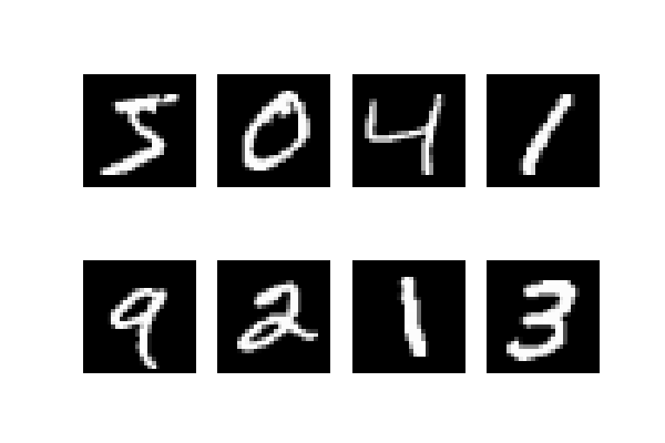
このチュートリアル通りに、mnistと呼ばれる手書き数字の画像分類をやってみます。
データセットを取得し、学習データとテストデータに分類します。
xが画像、yがラベルなので、yは 0-9 の数字です。
import tensorflow as tf

mnist = tf.keras.datasets.mnist
(x_train, y_train), (x_test, y_test) = mnist.load_data()

print('len(x_train): {}' .format(len(x_train)))
print('type(x_train): {}' .format(type(x_train)))
print('x_train.shape: {}' .format(x_train.shape))
# len(x_train): 60000
# type(x_train): <class 'numpy.ndarray'>
# x_train.shape: (60000, 28, 28)

print('len(x_test): {}' .format(len(x_test)))
print('type(x_test): {}' .format(type(x_test)))
print('x_test.shape: {}' .format(x_test.shape))
# len(x_test): 10000
# type(x_test): <class 'numpy.ndarray'>
# x_test.shape: (10000, 28, 28)

print('len(y_train): {}' .format(len(y_train)))
print('type(y_train): {}' .format(type(y_train)))
print('y_train.shape: {}' .format(y_train.shape))
# len(y_train): 60000
# type(y_train): <class 'numpy.ndarray'>
# y_train.shape: (60000,)

print('len(y_test): {}' .format(len(y_test)))
print('type(y_test): {}' .format(type(y_test)))
print('y_test.shape: {}' .format(y_test.shape))
# len(y_test): 10000
# type(y_test): <class 'numpy.ndarray'>
# y_test.shape: (10000,)
GPU が搭載されていない PC で実行するとcudaのdllが見つからないエラーが出ますが、問題ないので気にしないでください。
Could not load dynamic library 'cudart64_110.dll'; dlerror: cudart64_110.dll not found
mnistが 28×28 の白黒画像で、60,000枚の学習データと10,000枚のテストデータで構成されていることがわかりました。
何枚か画像にしてみましょう。
import matplotlib.pyplot as plt
from PIL import Image

rows = 2
cols = 4
fig, axes = plt.subplots(rows, cols, figsize=(6, 4))
for r in range(rows):
    for c in range(cols):
        img = Image.fromarray(x_train[r*cols+c])
        axes[r][c].imshow(img, cmap='gray')
        axes[r][c].axis('off') # 軸目盛りを消す。
filename = 'mnist_{}x{}_{}.png' \
    .format(rows, cols, datetime.now().strftime('%Y%m%d'))
file_path = os.path.join(os.getcwd(), filename)
fig.savefig(file_path)
モデルの構築と学習
Sequential モデルでネットワーク層を構築します。
https://keras.io/ja/getting-started/sequential-model-guide/
最後の層は、Dense で出力の次元を 10クラス とし、さらに活性化関数 softmax で、入力画像がどのクラスに所属するかの確率をそれぞれ出力し、すべての出力の合計が1となるようにします。
損失関数の from_logits=False にしているのは、モデルの出力が logits テンソルではなく、softmax 出力だからです。
ロジットの説明は こちらをご覧ください。
DeepL で翻訳すると、
分類モデルが生成する生の(正規化されていない)予測値のベクトルで、通常、正規化関数に渡される。モデルがマルチクラス分類問題を解く場合、ロジットは通常ソフトマックス関数への入力となる。とのことです。
model = tf.keras.models.Sequential([
    tf.keras.layers.Flatten(input_shape=(28, 28)),
    tf.keras.layers.Dense(128, activation='relu'),
    tf.keras.layers.Dropout(0.2),
    tf.keras.layers.Dense(10, activation='softmax')
])

# 損失関数
loss_fn = tf.keras.losses.SparseCategoricalCrossentropy(
    from_logits=False)

# compileで、損失・メトリック、オプティマイザを指定する。
model.compile(
    optimizer='adam',
    loss=loss_fn,
    metrics=['accuracy'],
    )

# 学習
history = model.fit(
    x_train,
    y_train,
    validation_split=0.2,
    epochs=10,
    batch_size=32,
    verbose=1,
    )
コマンドラインに学習の進捗具合が出力されます。
Epoch 1/10
1500/1500 [==============================] - 3s 2ms/step - loss: 2.8785 - accuracy: 0.7364 - val_loss: 0.5680 - val_accuracy: 0.8658
Epoch 2/10
1500/1500 [==============================] - 3s 2ms/step - loss: 0.6532 - accuracy: 0.8314 - val_loss: 0.4682 - val_accuracy: 0.9018
Epoch 3/10
1500/1500 [==============================] - 3s 2ms/step - loss: 0.5234 - accuracy: 0.8605 - val_loss: 0.3451 - val_accuracy: 0.9185
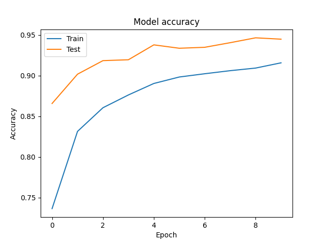
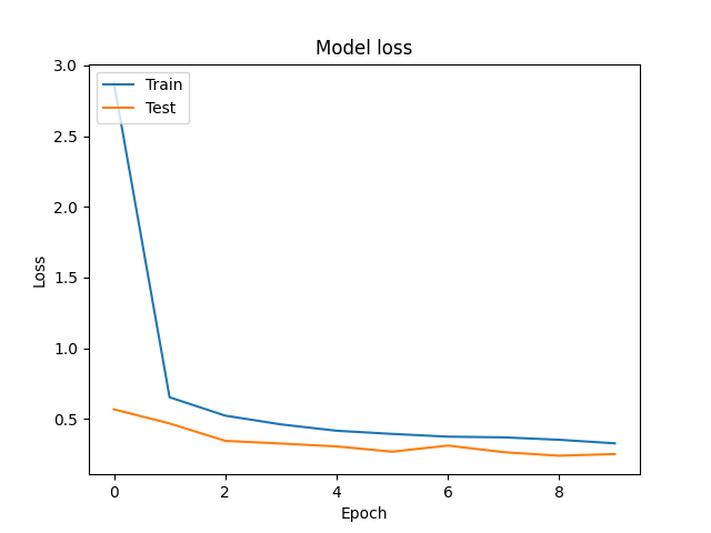
学習曲線を描いてみます。
Epoch が進むにつれて損失が収束していることがわかります。
# 学習の可視化
plt.plot(history.history['accuracy'])
plt.plot(history.history['val_accuracy'])
plt.title('Model accuracy')
plt.ylabel('Accuracy')
plt.xlabel('Epoch')
plt.legend(['Train', 'Test'], loc='upper left')
filename = 'accuracy_curve_{}.png' .format(datetime.now().strftime('%Y%m%d'))
file_path = os.path.join(os.getcwd(), filename)
plt.savefig(file_path)
plt.clf()
plt.close()

plt.plot(history.history['loss'])
plt.plot(history.history['val_loss'])
plt.title('Model loss')
plt.ylabel('Loss')
plt.xlabel('Epoch')
plt.legend(['Train', 'Test'], loc='upper left')
filename = 'loss_curve_{}.png' .format(datetime.now().strftime('%Y%m%d'))
file_path = os.path.join(os.getcwd(), filename)
plt.savefig(file_path)
plt.clf()
plt.close()
モデルの評価
学習に使用していないテストデータを使って、学習済みモデルが画像分類が正しくできてるか、評価します。
# 学習に使用していないテストデータで評価する。
results = model.evaluate(x_test, y_test, verbose=2)
print('Test loss: {:.6f}   Test accuracy: {:.6f}'
    .format(results[0], results[1]))
313/313 - 0s - loss: 0.2614 - accuracy: 0.9415 - 473ms/epoch - 2ms/step
Test loss: 0.261413 Test accuracy: 0.941500
94% くらいの精度が出ていることがわかりました。
いくつかのテストデータの、予測値と実際のラベルを見てみましょう。
# 予測
predictions = model.predict(x_test[:3])
# 指数表記にせず、小数点以下の桁数を指定する。
np.set_printoptions(suppress=True, precision=2)
print(predictions)
print(y_test[:3])
[[0. 0. 0. 0. 0. 0. 0. 1. 0. 0.]
[0. 0. 1. 0. 0. 0. 0. 0. 0. 0.]
[0. 1. 0. 0. 0. 0. 0. 0. 0. 0.]]
[7 2 1]
予測は 10クラス の内、0 から 9 になる確率がそれぞれ出力されています。
y_test ラベルは、x_test 画像の正解の数字です。
確率が最も高い数字と、正解の数字が合っていることがわかります。
以上が、機械学習の環境構築と簡単な学習例となります。
機械学習の実装は難しいということはなく、モジュールを使って簡単に作れることを感じていただけたと思います。
